The post explains how to obtain local deformation history from ABAQUS finite element simulation of a deformation process for modeling of the corresponding texture evolution by VPSC.

Intro

Simulations of texture evolution during simple monotonic loading (e.g. uniaxial tension, compression) can be readily performed with the stand-alone VPSC code. However, it is frequently desired to analyze texture evolution during complex non-monotonic deformation: for example, local texture evolution in a region of the sample during metal forming. In such cases, deformation histories can be obtained from finite element simulations. The present post describes a framework (inspired by Li et al., 2004) for obtaining local deformation histories from ABAQUS simulations of a deformation process in a format readable by VPSC. The calculation of the velocity gradient tensor needed for VPSC simulations is implemented in a user material subroutine (UMAT), whereas post-processing of the results and writing it to an output text file is performed with the aid of ABAQUS Python scripting.

Algorithm

For an ABAQUS/Standard simulation of a metal forming process with a simple and widely used J2 plasticity model and isotropic hardening, local deformation history can be obtained in the following steps.

1. Download my abaqus2vpsc.zip package containing the UMAT subroutine file (j2isoVelOut.for) and the Python script (abaqus2vpsc.py) for post-processing and extract it to a convenient location.
2. Create an ABAQUS/Standard model of the deformation process of interest as usual (create and mesh parts, define boundary conditions and interactions, etc.) with the following peculiarities:
   • Material. Create a user material with 22 solution-dependent variables (SDVs) and list Young modulus, Poisson ratio, and stress–strain data in Mechanical Constants table.
   • Field Output. Request field output for SDVs in the deformable part of interest with a a reasonable frequency that will guarantee sufficiently small time increment in the VPSC simulation.
   • UMAT file. Upon job creation, point to the UMAT subroutine file j2isoVelOut.for, which includes calculation of the velocity gradient tensor.
3. Run the ABAQUS/Standard simulation and make sure it is successfully completed.
4. Get the label of the element for which local texture evolution (and thus the deformation history) is of interest.
5. Run the Python script abaqus2vpsc.py from ABAQUS/CAE or command line, which will extract the components of the velocity gradient for the element of interest and write them to a text file.

Below are some details on these steps assuming usage of ABAQUS/CAE.

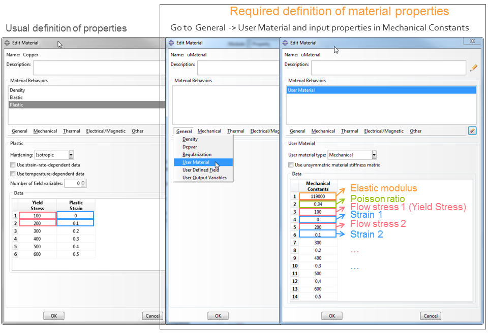
Creating user material

1. Create a new material, giving it a meaningful name.
2. Go to General -> User Material and list consequently elastic modulus, Poisson ratio, and flow stress–plastic strain pairs.
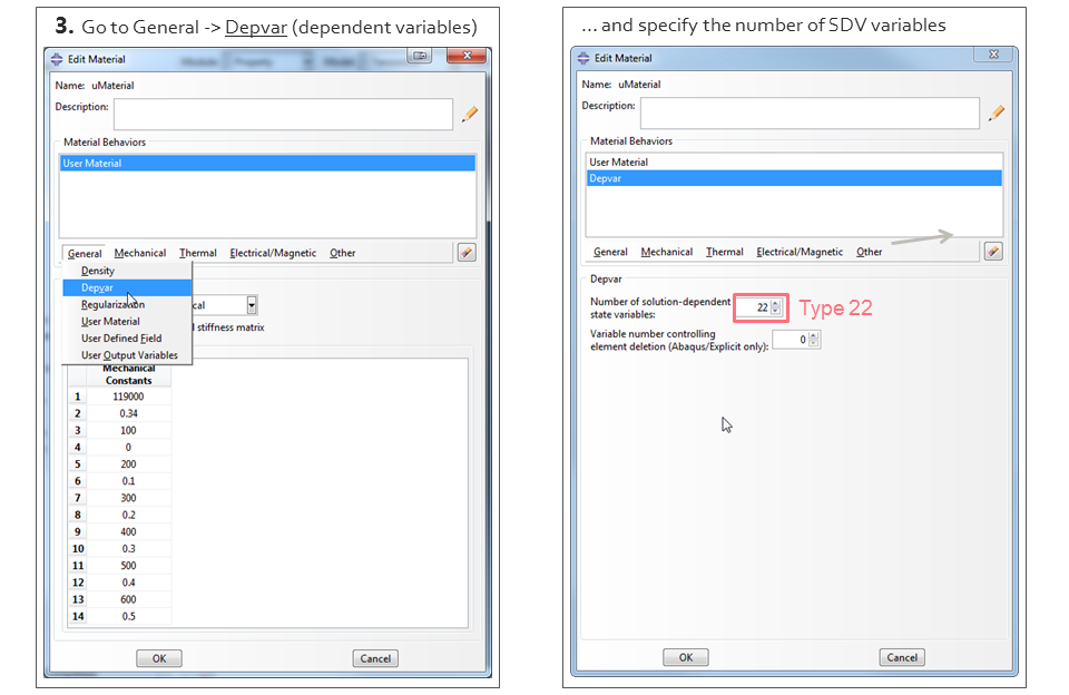
3. Go to General -> Depvar and set Number of solution-dependent variables to 22.

Tip: entry of stress–strain pairs to Mechanical Constants table might be really tedious when the number of data points is large. If you already have a “normally” defined material in your model tree, you may use elasplas2umat.py utility script (coming with abaqus2vpsc.zip package), which will transfer elastic and plastic properties from conventionally defined material to the Mechanical Constants of the user material.

Running ABAQUS simulation

After finalizing the finite element model, create a job and specify the path to j2isoVelOut.for in User subroutine file field in General tab of Edit job window. After pointing to the UMAT file, the job is ready for submission.

Identifying the element of interest

The Python script, which reads the components of the velocity gradient tensor from the ABAQUS output database (odb file), requires the label of the element for which the deformation history is needed. The label of the element can be found in the Mesh module of ABAQUS/CAE:

1. Go to Mesh module.
2. Go to Tools -> Query and choose Element
3. Pick the element for which local deformation history is needed
4. Read the label of the element of interest in the message area of ABAQUS window.

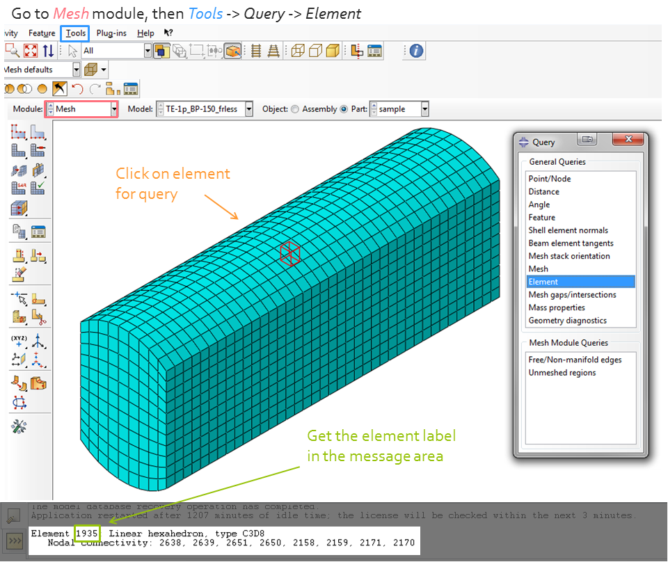Illustration of how to get the element label of interest in ABAQUS/CAE.

Post-processing

After running the simulation as described above, the components of the velocity gradient tensor can be accessed in the output database (odb file) as state variables (SDV). While it is possible to manually export these variables to a text file for subsequent use in VPSC, a Python script was developed for extracting the evolution of the velocity gradient with ease and in the right format for VPSC.

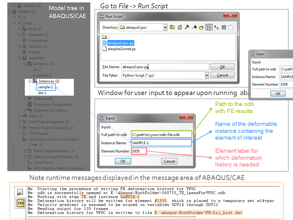
To run the script, open ABAQUS/CAE and

1. Go to File -> Run Script…, navigate to abaqus2vpsc.py file contained in the downloaded abaqus2vpsc.zip package.
2. In the appeared window for input, specify
   • the full path to the odb (e.g. C:\Temp\rolling.odb)
   • Instance name of the deformable sample (e.g. PART-1)
   • Element Number (or label) identified as described in the previous subsection
3. Check run-time messages of the script in the message area of ABAQUS/CAE. Particularly, check if Step, Instance, and Element number are correct. If the script completed successfully, the final message should be ‘Deformation history for VPSC is written to file same-path-as-odb\FE-Lij_hist.dat ’ (see figure below).

Running abaqus2vpsc.py script from ABAQUS/CAE with an example of filling the required fields.

As a result of running the script, the resulting file FE-Lij_hist.dat will contain a heading, steps, and the components of the velocity gradient in the format required by VPSC. This file can be readily used for VPSC simulations of the local texture evolution corresponding to the obtained local deformation history.

Running VPSC simulation

Refer to the VPSC manual on how to run a VPSC simulation of texture evolution for a given evolution of the velocity gradient tensor (especially Example 2, case B).

Appendix: Calculation of L tensor in UMAT

For texture simulations for non-uniform deformation, VPSC requires the evolution of velocity gradient tensor, $\mathbf{L}$. Since the velocity gradient tensor is not calculated in ABAQUS by default, its calculation has to be implemented in a user subroutine.

Why UMAT?

In the current framework, the calculation of the velocity gradient is implemented in UMAT subroutine for the following reasons:

• To UMAT, ABAQUS passes deformation gradient tensor, $\mathbf{F}$, from which the velocity gradient tensor can be readily calculated.
• UMAT allows for storing custom quantities (velocity gradient components in our case) in an array of state variables (or solution-dependent variables, SDVs), which are then accessible in the output database.

Furthermore, the main purpose of UMAT is to implement a custom constitutive model of the material so that the current framework can be used with a wide range of user-defined material models.

Calculation of the velocity gradient tensor

The velocity gradient tensor, $\mathbf{L}$, can be derived from the deformation gradient, $\mathbf{F}$, passed to UMAT as follows (Li et al., 2004)

where $\mathbf{F}_{t}$ and ${\mathbf{F}}_{\tau}$ are the deformation gradient tensors at the beginning and end of the time increment, $\Delta t$ is the time increment, and $\mathbf{I}$ is the identity tensor.

To implement the above equation in UMAT, we first calculate the inverse of the deformation gradient at the beginning of the time increment, $\mathbf{F}_{t}$, which is passed to UMAT as DFGRD0. To keep the main UMAT subroutine neat, we shall define and use a custom subroutine M3INV for calculation of the inverse of a 3x3 matrix:

CALL M3INV(DFGRD0,FTINV)

which results in that the inverse of the deformation gradient $\mathbf{F}^{-1}_{t}$ is stored in FTINV array.

We then calculate the product ${\mathbf{F}}_{\tau}{\mathbf{F}}^{-1}_{t}$, again using a custom subroutine MPROD.

CALL MPROD(DFGRD1,FTINV,AUX)

With the product ${\mathbf{F}}_{\tau}{\mathbf{F}}^{-1}_{t}$ being stored in an array AUX, we can finally calculate the velocity gradient tensor, $\mathbf{L}$, with the following snippet:

DO 231 I=1,3
	DO 231 J=1,3
		VELGRD(I,J) = (AUX(I,J)-ONEMAT(I,J))/DTIME
231   CONTINUE

To make the velocity gradient tensor accessible in the output database, we store $L_{ij}$ components to the array of state variables, or SDV, as (starting from index 14 because elements of STATEV with smaller indices are already in use for the constitutive model)

STATEV(14) = VELGRD(1,1)
STATEV(15) = VELGRD(1,2)
STATEV(16) = VELGRD(1,3)
STATEV(17) = VELGRD(2,1)
STATEV(18) = VELGRD(2,2)
STATEV(19) = VELGRD(2,3)
STATEV(20) = VELGRD(3,1)
STATEV(21) = VELGRD(3,2)
STATEV(22) = VELGRD(3,3)  

The code snippets presented above result in that, with proper field output request, the components of the velocity gradient tensor are accessible in the output database of the ABAQUS simulation. The calculation presented above can be incorporated into any UMAT subroutine for any material model as the computation requires only deformation gradient, which is always passed to UMAT by ABAQUS. Incorporation of the described computations in a UMAT subroutine requires care with the allocation of arrays (VELGRD FTINV, etc.). The example UMAT described in this post can be used as a reference for the right allocation of arrays. The utility subroutines M3INV, MPROD are also given there.