This article describes a procedure for generating ABAQUS finite element mesh from experimental EBSD maps using MTEX toolbox in MATLAB.

Introduction

It is sometimes desired to perform micromechanical finite element (FE) analysis of deformation of microstructures based on experimentally measured EBSD maps. The present post describes MATLAB scripts developed for automatic generation of FE mesh for a given EBSD map. The script is easy to use and requires minimal knowledge of coding in MATLAB.

To use the framework described here, you will need

• MATLAB
• MTEX toolbox
• ebsd2abaqus script (available on GitHub here)

Mesh generation

If you know how to use MTEX for EBSD analysis and have a clean EBSD map loaded into MATLAB that satisfies the following requirements:

• square grid
• no missing pixels

then download ebsd2abaqus script and generate the FE mesh with a single MATLAB command:

ebsd2abaqus(ebsd,angle)

where ebsd is a MATLAB variable containing the 2D EBSD data of interest and angle is the disorientation angle for grain segmentation.

The script takes EBSD pixels to form hexahedral elements of type C3D8 and writes the node coordinates to inp file. Grains are passed to ABAQUS as Element Sets, phases are passed as Element Sets and Sections, which makes it easy to assign different properties to grains or phases. Nodes on each face of the mesh are also saved as Node Sets that can be used to prescribe boundary conditions. The script generates pseudo-2D mesh: the resulting mesh consists of 3D elements but has only one element in thickness (along $z$ axis).

As a result of running the script, the mesh is written to ebsd.inp file. To work with the model, open ebsd.inp in ABAQUS/CAE by going File-Import-Model (or modify the input file directly in your favorite text editor). Define ABAQUS materials for each phase and finalize the finite element model (Step, BCs, etc.) to run the simulations.

If you are new to MTEX and unsure how to process the EBSD data, read on the following sections, which will guide you through the steps that might be necessary for preparing the data and correct mesh generation, such as

• EBSD data import
• conversion from hexagonal to square grid
• clean-up of inaccurate pixels
• filling missing pixels

EBSD data import

The current framework utilizes MTEX functions so that MTEX must be properly installed in MATLAB. MTEX is an open-source MATLAB toolbox for texture and EBSD analysis (available at http://mtex-toolbox.github.io/).

Once MTEX is installed, you need to import the EBSD data into MATLAB. If you have never used MTEX, the simplest way to import the data is through MTEX Import Wizard. Import Wizard can be started by typing import_wizard in MATLAB command window, which results in a window shown in the figure below.

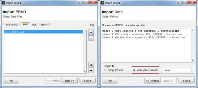
Go to EBSD tab and click +. Browse to your EBSD file and open it. Accept the default settings in several windows, choose workspace variable as the import method in Import Data window and push Finish. Now EBSD data is stored in a variable ebsd. Further data processing will be carried out on this variable.

Pre-processing

Grid conversion

The present framework of building a FE model approximates microstructures by hexahedral mesh, i.e. mesh consisting of cuboidal (C3D8) elements. The use of a hexahedral mesh inevitably leads to ladder-like grain/phase boundaries, however, this is assumed to be a sufficiently good approximation for many cases, especially when the EBSD map has a relatively high resolution.

Building a hexahedral mesh is much easier if the EBSD data is on a square grid. Since experimental EBSD maps are frequently recorded on hexagonal grids, it is necessary to convert these maps to square grids. In MTEX conversion can be done by using fill function:

ebsd = fill(ebsd)

Pro-tip: Although fill(ebsd) converts the grid, use this function with care and check if the data is not distorted. If the results of fill function are not satisfactory, you can also try converting grids in ang files prior to loading the data into MTEX with the aid Dream.3D software (available at http://dream3d.bluequartz.net/). Have a look at Convert Hexagonal Grid Data to Square Grid Data filter, which also allows for batch conversion of many files.

Clean-up

Experimental EBSD maps often contain inaccurate pixels which are undesirable in the FE model to be generated. The following pixels can be considered as “undesirable”:

• non-indexed pixels
• pixels with low confidence index (CI)
• pixels that belong to unreasonably tiny “grains” (which result in the presence of numerous grains that consist of only one or two pixels)

Non-indexed and low-quality pixels can be removed with the following lines:

ebsd('nonIndexed') = [];
ebsd(ebsd.ci < minCI) = [];

where minCI is the threshold CI such as 0.1.

Getting rid of pixels that belong to unreasonably tiny “grains” require prior grain segmentation:

[grains,ebsd.grainId,ebsd.mis2mean] = calcGrains(ebsd,'angle',angle*degree);

with angle being the disorientation angle for thresholding grains (e.g. 15).

After grain segmentation, such “bad” pixels can be removed as follows:

indSmallSize = grains.grainSize < minSize;
ebsd(grains(indSmallSize)) = [];

Automating the clean-up

Since we are likely to do some clean-up routine over and over again, it is a good idea to put such routine to a separate function.

As an example, I organized my cleaning routine into a function called clean4fem (available on GitHub here). This function excludes the “bad” pixels mentioned above – non-indexed, with low CI, and of tiny grains. In addition, the script fills the removed pixels with phase ID, grain ID, and orientations equal to those of the grain surrounding these removed pixels.

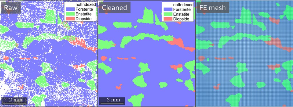
Finally, for control purposes, the script plots three maps: raw EBSD data, data with inaccurate pixels removed, and finally the cleaned map with filled pixels (see Example section).

Typical use of this function will be as follows:

ebsd = clean4fem(ebsd,minSize,minCI,angle);

where minSize – is the size of the grain in pixels below which grains are considered unreasonable, minCI – min confidence index to keep, angle – disorientation angle for grain segmentation.

Crop

Sometimes only a certain region of EBSD map is of interest for FE analysis. In such cases, EBSD maps can be cropped by logical indexing based on coordinates.

For example, if the EBSD map is 30 $\mu m$ along $x$ and 15 $\mu m$ along $y$ and suppose only one half (along $x$) of the map is of interest, the map can be cropped by the following commands:

ebsd = ebsd(ebsd.x >= 15);

A more arbitrary region can be also cropped:

region = [x0 y0 dx dy];
condition = inpolygon(ebsd,region);
ebsd = ebsd(condition);

Refer to MTEX manual to learn more about selecting a certain region.

Pro-tip: it is a good idea to do cropping first of all because it will save a lot of computational cost: any processing is much faster on a smaller map!

Example

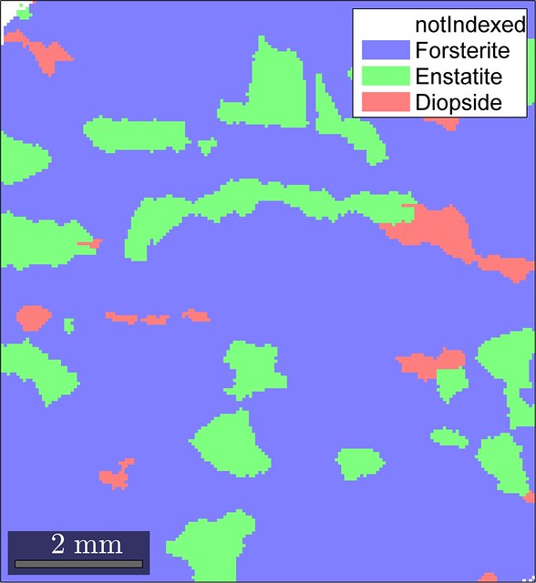
Let’s try the workflow described above on realistic EBSD data, for example, on Forsterite dataset pre-packaged with MTEX.

Loading the data

To load the Forsterite dataset, simply run the following in MATLAB command line:

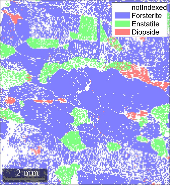
mtexdata forsterite

As a result of this command, the raw EBSD data is loaded into variable ebsd, whose visualization using

plot(ebsd)

will look as shown below.

Here we can see a high-resolution map with several phases and many non-indexed pixels. A perfect dataset to test our framework!

Cropping the map

The loaded EBSD map has 245,952 pixels, which is a bit overwhelming for FE analysis so let’s crop the EBSD map, say, to a quarter of the original map along $x$ axis and to a half along $y$:

ebsd = ebsd(ebsd.x >= 3*max(ebsd.x)/4);
ebsd = ebsd(ebsd.x >= max(ebsd.y)/2);

Cleaning-up

Now let’s clean our map using the mentioned helper function clean4fem, with the following settings:

• minimum allowed quality: mad = 0.1;
• minimum allowed grain size: 5 px;
• disorientation angle for grain segmentation: 15 degrees.

This can be accomplished with the following command (provided clean4fem is placed into MATLAB path)

ebsd = clean4fem(ebsd,5,0.1,15.0)

The changes that the EBSD map undergoes are shown in the figure below.

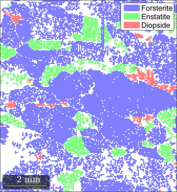
Looks like our cleaning routine did not produce significant artifacts (at least in terms of the phase distribution) and resulted in a reasonable final EBSD map so that we can move on to mesh generation.

Mesh generation

Now our EBSD data is ready for mesh generation, which, after downloading ebsd2abaqus script, is as simple as

ebsd2abaqus(ebsd,angle)

where, again, angle is the disorientation angle in degrees for grain segmentation, e.g. 15.

Caveat: pass the segmentation angle without degree variable, i.e. for angle of 15 the function call is ebsd2abaqus(ebsd,15.0), just like in the case of clean4fem function.

Data checks in ebsd2abaqus

An important thing to keep in mind is that the script performs two checks of the data

1. Whether or not EBSD is on hexagonal grid
2. Whether or not EBSD has non-indexed pixels

If any of these conditions are true, the script will call MTEX function fill to convert the data to a square grid or to fill the non-indexed pixels. The script will inform the user if the fill function was used and which of the conditions (grid or non-indexed pixels) was the reason.

For example, despite cleaning with clean4fem function, our EBSD map of forsterite still had some non-indexed pixels at the corners of the map and ebsd2abaqus displayed the following warning message

WARNING! EBSD had 54 non-indexed pixels and so was filled using fill function

Since it is only 54 pixels located at the corners, the final EBSD map should be fine and we can use the generated mesh for simulations. However if there are many non-indexed pixels (e.g. when the script is used without prior cleaning), it is better to check if the EBSD map after filling does not have significant artifacts.

Similarly, if we feed an EBSD map measured on hexagonal grid to ebsd2abaqus, the script will automatically convert it to a square grid using the same fill function and show a warning:

WARNING! EBSD was on hex grid and so was converted to sqr grid using fill function

If this is the case, again, it is worth checking if the use of fill function does not lead to significant distortions in the EBSD data.

The mesh in ABAQUS/CAE

The generated ebsd.inp contains the following

• Mesh (nodes and elements)
• Element Sets for grains and phases
• Sections for phases

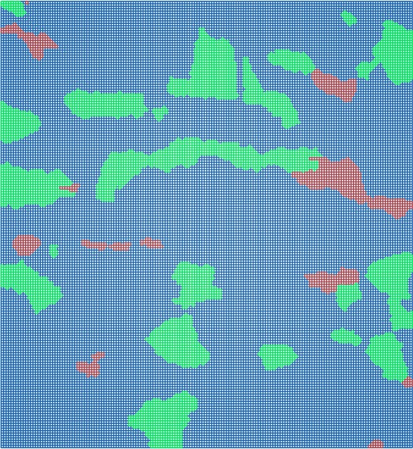
In ABAQUS/CAE, the generated mesh consisting of 30,744 C3D8 elements looks as shown below.

Whereas the model tree in ABAQUS/CAE looks like this:

Parts
└── SAMPLE
    └── Sets
    	├── ALLELEMENTS           # Element set containing all the elements
    	├── ALLNODES              # Node set containing all the nodes
    	├── GRAIN-1               # Element set constituting GRAIN-1
    	├── GRAIN-2               # Element set constituting GRAIN-2
    	├── ...                   # etc.
    	├── NODES+1               # Node set containing nodes on the face of +X
    	├── NODES+2               # Node set containing nodes on the face of +Y
    	├── NODES+3               # Node set containing nodes on the face of +Z
    	├── ...                   # etc.
    	├── PHASE-DIOPSIDE        # Element set constituting phase diopside
    	├── PHASE-ENSTATITE       # Element set constituting phase enstatite
    	└── PHASE-FORSTERITE      # Element set constituting phase forsterite
Materials                         # Create materials with phase names as material names
Sections                          # Sections for phases
	├── Section-1-PHASE-FORSTERITE
	├── Section-2-PHASE-ENSTATITE
	└── Section-3-PHASE-DIOPSIDE

Step                              # Create step, BCs, etc.
...

The sections for phases are created assuming that there will be a material for each phase so that for this model we need to create three materials: Forsterite, Enstatite, and Diopside with the desired properties. Finally once we define all the other ingredients – step, boundary conditions, output, we are ready to run the microstructure-based simulations!

Citation

The script presented here is a by-product of one of my short-term research projects – on medium manganese steel – while I was at POSTECH. You can find the publication resulting from this project (and showing ebsd2abaqus in action) here. Feel free to cite the paper (or even this post) if you like.

Bibtex entry:

@article
{Latypov2016,
author = {Latypov, M.I. and Shin, S. and {De Cooman}, B.C. and Kim, H.S.},
doi = {10.1016/j.actamat.2016.02.001},
issn = {13596454},
journal = {Acta Materialia},
keywords = {Finite element methods,Medium Mn steel,Strain partitioning,TWIP+TRIP},
pages = {219--228},
title = { {Micromechanical finite element analysis of strain partitioning in multiphase medium manganese TWIP+TRIP steel} },
volume = {108},
year = {2016}
}

Acknowledgements

Thanks are due to Ralf Hielscher for explanations on grid checks and conversion.