This post is a short tutorial to help getting started with crystal plasticity simulations of texture evolution during plastic deformation. It explains how to run a simple VPSC simulation and visualize the simulated texture in MTEX.
Intro
While VPSC comes with a manual that exhaustively treats the theory and usage of the software, all the details given there may look overwhelming for a beginner. This post is an attempt to aid running VPSC for the first time. It is assumed that the reader has a working VPSC7 executable and an access to MATLAB with MTEX (ver. 4.0.2x or later) installed.
Input
Running a VPSC simulation requires several input files. The VPSC manual gives a detailed line-by-line description of each of the input files so that only a very brief overview is given here for a minimal set of input files required for running a simple simulation. The simulation described in this tutorial follows Example 1 (Uniaxial tension of fcc steel) of the manual and all the necessary files should be available in VPSC package.
-
Master input file,
vpsc.in, is the main one. It contains the data on phases present in the aggregate, various simulation settings as well as pointers to the other input files. We are going to accept the settings given in Example 1 so that we only need to make sure that the paths to the other input files are correct. Note thatvpsc.inmust be in the same folder asvpsc.exe. -
Texture input file contains a set of Bunge Euler angles that represent the initial texture. VPSC offers
rand500.texfile with a set of 500 random orientations, which is sufficient for runing a simple simulation. -
Single crystal input file contains crystal symmetry, elastic stiffness, slip and twinning systems, the hardening law and hardening parameters. We will use an input file for fcc austenitic steel deforming by slip only and with no strain hardening (provided as
fcc.sxin VPSC and shown on p. 55 of the manual). -
Boundary conditions input file specifies velocity gradient tensor and Cauchy stress tensor. The components of the velocity gradient and stress tensors are enforced through binary matrices
IUDOTandISCAU, respectively (1 is on, 0 is off). In Example 1, uniaxial tension in direction is defined through a velocity gradient tensor with , , and zero off-diagonal components. Since we enforce the velocity gradient here, all components ofIUDOTare 1, whereas all components ofISCAUare 0. Finally, uniaxial tension in this example is performed up to von Mises strain of 1.0 in 50 increments, which is specified in the first line of the BC input file.
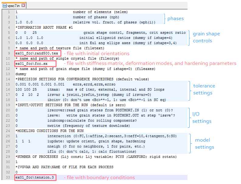 A screenshot of
 vpsc.in file provided for Example 1 (should be available as vpsc7in.t in ex_01_FCC folder).
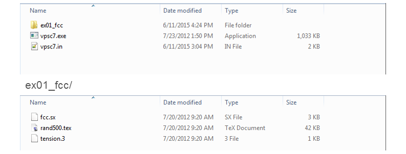 Illustration of arrangement of the input files that corresponds to the
 vpsc.in shown above.
Running the simulation
On Windows, VPSC simulation can be launched by just a double click on vpsc.exe. However, to be able to see runtime (or error) messages after simulation is completed (or failed), it is worth launching the simulation from Command Line.
Tip: for a quick access to Command Line in the current folder, hold Shift button and right-click anywhere in the folder. Press ‘Open command window here’ in the context menu and there will be no need in ‘cd’-ing all the way down to your current location.
Output
Upon successful completion of the simulation, there will be several output files. Again, the VPSC manual explains each of them in detail. In this tutorial, we will focus only on stress–strain curves and texture output.
Stress–strain curves
Strain and stress tensors as well as von Mises stress and strain are written to STR_STR.OUT file. The von Mises values are the first two columns in the file and can be easily plotted in any software.
Texture visualization
Texture output from VPSC is written to TEX_PH1.OUT file. There are different texture packages that can be used to visualize the simulated texture: from pole8 coming with VPSC to commercial software LaboTex.
This tutorial demonstrates texture visualization in free and open-source MATLAB toolbox MTEX.
If MTEX is properly installed, the set of Euler angles obtained in VPSC can be loaded to MTEX by loadEBSD_generic function. To do that, we first specify the crystal symmetry of our material and point to the path of the texture file:
texFile = 'your-folder/TEX_PH1.OUT';
CS = crystalSymmetry('cubic');
and then load the data by calling loadEBSD_generic as
data = loadEBSD_generic(texFile,'CS',CS,'ColumnNames',{'Euler1' 'Euler2' 'Euler3'}, 'Bunge');Now our orientations are stored in a variable data. Since we loaded it using loadEBSD function, MTEX treats the variable as EBSD data even though there is no spatial information for the orientations. At any rate, the orientations can be easily accessed as
ori = data.orientations;Now we can readily plot these discrete orientations in a pole figure with plotPDF function. We only need to specify the Miller indices of the poles we would like to plot. In MTEX, Miller indices are defined by function Miller, e.g. Miller(h,k,l,CS). Then, for a (111) pole figure, the command will be
figure; plotPDF(ori,Miller(1,1,1,CS),'all')Tip: keyword ‘all’ in
plotPDFensures that all orientations are plotted; otherwise MTEX will plot only a randomly picked subset of the orientations to save memory.
The inverse pole figure can be plotted using plotIPDF function. For an inverse pole figure, we select a specimen direction to plot in respect to the crystal frame. Since tension in the simulation was performed in direction, it is reasonable to visualize distribution of the specimen direction, which can be accessed as zvector in MTEX. Then the command is
figure; plotIPDF(ori,zvector)Tip: inverse pole figure might be oriented in an unexpected way: (111) pointing west instead of north. To “fix” this, run command
plotx2eastprior to plotting or, in existing Figure window, go to MTEX -> X axis direction -> East.
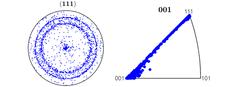 The result of plotting discrete orientations in a pole figure and inverse pole figure.
Next, to make continuous plots, we need to estimate orientation distribution function (ODF). In MTEX, ODFs can be calculated from a set of discrete orientations by calcODF function:
odf = calcODF(ori);Now that the ODF for our orientation set is stored in odf variable, we can plot pole figures and inverse pole figures using plotPDF and plotIPDF functions in the same fashion as for discrete orientations, i.e.
figure; plotPDF(odf,Miller(1,1,1,CS))
figure; plotIPDF(odf,zvector)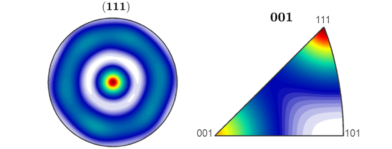 The result of plotting ODF in a pole figure and inverse pole figure.
Since Example 1 of the VPSC manual features predictions of texture and stresses with different interaction schemes: Full Constraint (aka Taylor), Affine, Secant, Tangent, and others, the reader is encouraged to run the simulations with these different settings and compare the predictions with those in the manual. The interaction schemes can be set in the main input file (vpsc.in) by choosing the desired value for interaction variable.
Custom function for VPSC texture
Once we set our mind on how we would like to visualize simulated textures and if we are to use the procedure repeatedly for many output data sets, it is handy to write a custom function that will do the whole thing with the file name as the only input from the user.
For our case such a function will be something like this (let’s call it plotVpscTex):
function plotVpscTex(fileName)

% crystal symmetry
CS = crystalSymmetry('cubic');
% pole figures to plot
h = [Miller(1,1,1,CS) Miller(0,0,1,CS) Miller(0,1,1,CS)];
% inverse pole figures to plot
r = [xvector yvector zvector];

data = loadEBSD_generic(fileName,'CS',CS,'ColumnNames',{'Euler1' 'Euler2' 'Euler3' 'weight'}, 'Bunge');
ori = data.orientations;

figure; plotPDF(ori, h,'all')
figure; plotIPDF(ori, r)

end
Note that, in this function, plotPDF and plotIPDF are used for h and r variables which contain several Miller indices and specimen directions. It allows plotting several pole figures and inverse pole figures at once and thus choosing the best one for visualization in each particular case. This function can be easily customized further for continuous or contour plots, etc.